

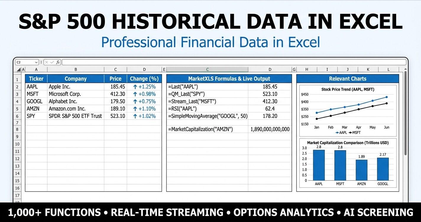
To get S&P 500 historical data in Excel with MarketXLS, use =Close_Historical("^GSPC","2020-03-23") for the index close on a date, =Adjusted_Close_Historical("SPY","2020-03-23") for a dividend- and split-adjusted SPY close, or =QM_GetHistory("SPY") to spill the full daily OHLCV history into a sheet. The same functions work on each of the 500 components, so a ticker list in column A plus one formula tiled across dates gives you component history too.
This guide covers both paths (the index and its components), return and sector-weight calculations, and why adjusted close matters. It links two templates: a static snapshot and a live MarketXLS workbook where every cell is a formula. On Mac or Excel for the web (the Microsoft 365 add-in), prefix the functions with mxls..
Quick Reference: The Functions You Will Use Most
These are the core MarketXLS functions used in both templates:
| Function | What it returns | Example |
|---|---|---|
| =QM_Last(Symbol) | Current last traded price or index level | =QM_Last("SPY") |
| =QM_GetHistory(Symbol) | Spill array of historical OHLCV | =QM_GetHistory("AAPL") |
| =CLOSE_HISTORICAL(Symbol, Date) | Close on a specific date | =CLOSE_HISTORICAL("^GSPC","2020-03-23") |
| =OPEN_HISTORICAL(Symbol, Date) | Open on a specific date | =OPEN_HISTORICAL("SPY","2024-01-02") |
| =HIGH_HISTORICAL(Symbol, Date) | Intraday high on a specific date | =HIGH_HISTORICAL("SPY","2024-01-02") |
| =LOW_HISTORICAL(Symbol, Date) | Intraday low on a specific date | =LOW_HISTORICAL("SPY","2024-01-02") |
| =ADJUSTED_CLOSE_HISTORICAL(Symbol, Date) | Split and dividend adjusted close | =ADJUSTED_CLOSE_HISTORICAL("AAPL","2020-08-31") |
| =VOLUME_HISTORICAL(Symbol, Date) | Share volume on a specific date | =VOLUME_HISTORICAL("SPY","2024-01-02") |
| =Sector(Symbol) | GICS sector classification | =Sector("AAPL") |
| =MarketCapitalization(Symbol) | Current market capitalization | =MarketCapitalization("AAPL") |
| =Beta(Symbol) | Beta versus market | =Beta("AAPL") |
| =DividendYield(Symbol) | Trailing dividend yield (decimal) | =DividendYield("XOM") |
Keep this list handy. The rest of this guide is mostly about combining these primitives into useful workbooks.
Two Different Questions, One Toolkit
"S&P 500 historical data" usually means one of two things: the index level over time, or the price history of its components. The workbook answers both.
The first interpretation is the index itself. The S&P 500 index uses the symbol ^GSPC for historical lookups in MarketXLS. The ETF SPY tracks the same index and is the usual reference when comparing to a portfolio that holds real shares; its adjusted close includes reinvested dividends, so it gives a total-return view. Either symbol works as the spine of your historical study.
The second interpretation is the components. The S&P 500 is a portfolio of 500 large-cap U.S. companies, and the index level is a market-cap-weighted aggregate of the prices of those 500 names. When a user wants to study earnings season, sector rotation, factor performance, or single-stock dispersion, what they really want is the historical data for the constituents, organized by sector, weight, and time window. MarketXLS supports this with the same historical functions applied across a watchlist of tickers.
Our templates handle both paths in the same workbook. The Index Snapshot sheet handles ^GSPC and SPY. The Components Watchlist and Historical Prices sheets handle the constituents. The Return Analysis and Sector Weights sheets connect the two so you can see how the index level decomposes into the underlying names.
Path One: S&P 500 Index Historical Data
For the index itself, put a date in cell B2, drop ^GSPC or SPY in cell A2, and reference both in your historical functions.
The most useful single formula is the adjusted close, because that is the figure that should drive return math:
=ADJUSTED_CLOSE_HISTORICAL("SPY","2020-03-23")
Formula documentation: ADJUSTED_CLOSE_HISTORICAL
That returns the dividend-adjusted closing level on the COVID-era low date. Pair it with QM_Last("SPY") and you have a total-return calculation:
=QM_Last("SPY") / ADJUSTED_CLOSE_HISTORICAL("SPY","2020-03-23") - 1
Formula documentation: QM_Last, ADJUSTED_CLOSE_HISTORICAL
^GSPC is a price index, so its history does not include reinvested dividends. For price-return analysis (for example "the S&P 500 is up X percent since 2020"), use ^GSPC, because it matches what financial media quote. For a total-return comparison, use SPY's adjusted close, because it reflects the dividends SPY pays out.
In our template, the Index Snapshot sheet shows both side-by-side so you can pick the right framing for the question you are answering.
Common Index-Level Levels to Pull
| Date | Why it matters | Formula |
|---|---|---|
| 2020-03-23 | COVID-era index low | =CLOSE_HISTORICAL("SPY","2020-03-23") |
| 2022-10-12 | Post-Fed-hike cycle low | =CLOSE_HISTORICAL("SPY","2022-10-12") |
| 2023-05-12 | Mid-cycle reference | =CLOSE_HISTORICAL("SPY","2023-05-12") |
| 2024-12-31 | Year-end 2024 close | =ADJUSTED_CLOSE_HISTORICAL("SPY","2024-12-31") |
| Five years ago | CAGR anchor | =ADJUSTED_CLOSE_HISTORICAL("SPY","2021-05-13") |
Each of those is a single cell in Excel, with no CSV download or manual cleaning. Use trading days: a weekend or holiday date may return no value.
Path Two: S&P 500 Component Historical Data
Component history needs a list of the constituents and the same historical lookups run for each ticker.
Our template assumes you already have a watchlist of names. You can paste in a sub-universe (top 15 by weight, an equal-weight sample, a sector slice) and the formulas will repoint automatically. If you want the full 500, the MarketXLS plugin has a downloadable list of S&P 500 members through its menu in the Excel ribbon, and you can copy that list into column A of the Components Watchlist sheet to drive everything below it.
Here is the structure on the Components Watchlist sheet:
A: Ticker (input)
B: =Sector(A4)
C: =Industry(A4)
D: =QM_Last(A4)
E: =SimpleMovingAverage(A4,"50")
F: =SimpleMovingAverage(A4,"200")
G: =FiftyTwo_WeekHigh(A4)
H: =FiftyTwo_WeekLow(A4)
I: =Beta(A4)
J: =DividendYield(A4)
Formula documentation: Sector, Industry, QM_Last, SimpleMovingAverage, FiftyTwo_WeekHigh, FiftyTwo_WeekLow, Beta, DividendYield
Edit a ticker in column A and every cell to the right repoints. The same pattern works for the Historical Prices sheet, where the same column of tickers gets paired with a reference date in cell B2 and OHLC formulas spill across the row.
For multi-date historical pulls, you can build a matrix instead of stacking dates vertically:
=ADJUSTED_CLOSE_HISTORICAL($A5, B$4)
Formula documentation: ADJUSTED_CLOSE_HISTORICAL
Where row 4 holds the dates as headers and column A holds the tickers. A single formula tiled across the rectangle gives you a clean grid of adjusted closes that you can chart or feed into a return calculator.
Working With the Full S&P 500
A few practical notes for analysts pulling the full constituent list:
-
The S&P 500 reconstitutes regularly. Names get added and removed. If you are looking far enough back, some of today's components were not in the index and some of yesterday's components are no longer there. For point-in-time studies, freeze the membership list on the date that anchors your analysis.
-
Some constituents have ticker variants (BRK.B, BF.B). MarketXLS supports these but make sure you use the exact symbol your data provider expects.
-
Adjusted close is your friend for return math, but raw close is what you want when comparing to a specific historical headline ("the S&P 500 closed at X on date Y"). Choose the right one for the question.
Return Analysis: Stitching It Together
The Return Analysis sheet in the template is where the index and the components share a frame. Each row is a ticker. Each column is a return window. The formulas are simple enough that you can read them in your head:
1Y Return: =QM_Last(A4)/ADJUSTED_CLOSE_HISTORICAL(A4,"2025-05-13")-1
3Y Return: =QM_Last(A4)/ADJUSTED_CLOSE_HISTORICAL(A4,"2023-05-12")-1
5Y Return: =QM_Last(A4)/ADJUSTED_CLOSE_HISTORICAL(A4,"2021-05-13")-1
CAGR 5Y:  =(1+5Y Return)^(1/5)-1
Formula documentation: QM_Last
This is the simplest possible return calculation: today's price divided by some prior adjusted close, minus one. Wrap each formula in IFERROR so a missing data point does not break the entire row. The template does this for you.
The component returns show dispersion: the headline S&P 500 return for any window hides a wide range of outcomes, with some names far ahead of the index and some negative. The template shows the index and component returns side by side.
Sector Weights: Why the Index Is Not Diversified the Way People Think
The Sector Weights sheet rolls the components up into GICS sectors, which shows how concentrated the index is.
The S&P 500 is market-cap-weighted, which means a small number of mega-cap names drive a disproportionate share of the index return. The Information Technology sector alone has been roughly 30 percent of the index in recent years. Add Communication Services (which holds GOOGL and META) and Consumer Discretionary (which holds AMZN and TSLA), and roughly half of the index sits in technology-adjacent businesses.
That has a few historical implications worth flagging in any analysis:
- Concentration is structural, not anomalous. Looking at the last 10 years of S&P 500 history, the mega-cap tech weighting has trended up, not down. Studies of historical S&P 500 returns should weight the contribution of the top names appropriately.
- Sector weights shift the index. When one sector swings from 30 percent to 25 percent of the index, the index level reflects that shift even if no individual stock collapsed. Historical sector weights are part of the index history, not just the component history.
- An equal-weight comparison tells a different story. The S&P 500 Equal Weight Index (RSP is the common ETF proxy) has historical returns that diverge meaningfully from the cap-weighted S&P 500 in certain windows. If your historical study is about market breadth, you may want to pull RSP history alongside SPY.
The template's Sector Weights sheet uses Sector(), MarketCapitalization(), and PERatio() to roll up the component data into sector-level statistics. A SUMIF on market cap by sector gives you the rough weight, and an AVERAGEIF on P/E ratio by sector gives you the valuation contour.
Building Your Own S&P 500 Historical Data Workbook From Scratch
If you want to build a workbook from scratch instead of starting from our template, here is the minimum viable structure that handles both the index and the components:
Sheet 1: Inputs
- A1: Index symbol (^GSPC or SPY)
- A2: Reference date for return base
- A3: List of component tickers (paste in your watchlist or the full 500)
Sheet 2: Index History
- For the index symbol, build a row per reference date.
- Use CLOSE_HISTORICAL, OPEN_HISTORICAL, HIGH_HISTORICAL, LOW_HISTORICAL, ADJUSTED_CLOSE_HISTORICAL.
- Add a return column using QM_Last over each historical close.
Sheet 3: Component History
- Tickers from Inputs roll into column A.
- For each ticker, pull OHLC at the reference date.
- Add a CAGR column and a 1Y/3Y/5Y return column.
Sheet 4: Sector Rollup
- Use Sector(A) on each component to get the GICS sector.
- SUMIF on market cap by sector for weights.
- AVERAGEIF on returns by sector for sector-level historical performance.
Sheet 5: Charts
- One line chart of the index over time (use QM_GetHistory as a spill source).
- One bar chart of component returns sorted high to low.
- One donut chart of sector weights.
That is the skeleton. Everything else (correlation, drawdown, rolling volatility, factor decomposition) is a layer on top of these five sheets.
Adjusted Close Versus Raw Close: A Detail That Matters
For return math on S&P 500 components, use ADJUSTED_CLOSE_HISTORICAL, not CLOSE_HISTORICAL. Adjusted close accounts for stock splits and dividends, so a ratio of two adjusted closes gives you a total return. A ratio of two raw closes can mislead you, sometimes severely, for any name that has paid dividends or split shares over the period.
A worked example: Nvidia had a 10-for-1 split on 2024-06-10. If you compute a return by dividing today's QM_Last by CLOSE_HISTORICAL of any date prior to that split, the result is roughly one-tenth of the true figure, because the historical close is on the pre-split share scale (about 10 times higher). ADJUSTED_CLOSE_HISTORICAL handles the adjustment for you and produces a clean total return.
The same applies to dividends. Energy names like XOM have paid yields of roughly 3 percent. Over five years that compounds into a 15 to 20 percent dividend contribution to total return. A raw price return understates the picture. Adjusted close is the right reference for return math.
The only time you want raw close is when you are reproducing a headline number or aligning with a specific historical chart. For everything else, adjusted close.
A Note on Data as of Dates
Whenever you publish or share an S&P 500 historical data workbook, stamp it with a "Data as of" date. Our sample template includes this on the How To Use sheet and on the Index Snapshot dashboard. The reason is that QM_Last refreshes when the workbook recalculates (15-minute delayed on the Standard plan, real-time on Advanced and Business), but the historical numbers in the sample (the snapshot file) are frozen at the moment of publish. If you forget to time-stamp, anyone who opens the file in three months will assume the static values are current, and that creates the kind of small-but-real reporting errors that erode trust over a long relationship.
The template version is different: every cell is a formula, so the workbook recalculates on open. There is no "data as of" risk because there is no static data.
Charting Five Years of S&P 500 History From a Single Formula
=QM_GetHistory returns a symbol's OHLCV history as a spill array from a single formula:
=QM_GetHistory("SPY")
Formula documentation: QM_GetHistory
That spills into a grid of date, open, high, low, close, volume, and adjusted close. Highlight the date column and the adjusted close column and insert a line chart. You now have a multi-year S&P 500 chart that updates automatically when you refresh.
For component-level charts, the same pattern works:
=QM_GetHistory("AAPL")
Formula documentation: QM_GetHistory
You can stack these on separate sheets and reference them from a master chart sheet using INDEX or named ranges. For a true index decomposition view, pulling QM_GetHistory for each top component and stacking the adjusted closes lets you watch dispersion accumulate over time.
Frequently Asked Questions
What ticker should I use to pull S&P 500 historical data in Excel?
For the index level, use ^GSPC. For a total-return view, use SPY's adjusted close, which reflects the dividends SPY pays. For an equal-weight comparison, use RSP. To match a headline such as "the S&P 500 closed at X," use ^GSPC.
How far back does the historical data go?
SPY began trading in 1993, so SPY history starts there. The S&P 500 index itself has a much longer history. Component data starts no earlier than each stock's listing date. Check the start date MarketXLS returns for your symbol with =QM_GetHistory before relying on a very long window.
Can I pull historical data for all 500 S&P 500 components at once?
Yes. Paste the constituent list into column A of a sheet and tile your historical formulas across the rows. Performance depends on how many cells you are computing simultaneously; for full-universe pulls across long histories, refresh in segments rather than all at once.
How do I handle index reconstitution when pulling historical data?
The S&P 500 changes its constituents over time. For point-in-time analysis, freeze the membership on your anchor date. The MarketXLS plugin's S&P 500 list is the current membership; for historical membership at a prior date, you would need a survivor-bias-free roster from a specialized data provider.
Why are my historical returns different in raw close versus adjusted close?
Adjusted close accounts for stock splits and dividends. Raw close does not. For total return analysis on any name that has paid dividends or split, always use ADJUSTED_CLOSE_HISTORICAL. Raw close is for matching historical headlines or specific point-in-time charts.
Can I build a custom S&P 500 sector tracker with MarketXLS?
Yes. Use Sector() on each component, SUMIF on MarketCapitalization() to compute sector weights, and chain historical price functions over a date range to compute sector-level returns. The Sector Weights sheet in our template is a starting point.
Download the Templates
Both files are linked below. The sample file is a static snapshot you can open and read immediately. The template file is the live MarketXLS workbook where every cell is a formula.
Download the templates:
- - Pre-filled with current data and full formula notes
- - Live-updating formulas across index, components, and sector rollup
Open the template file with MarketXLS installed in Excel, hit refresh from the MarketXLS ribbon, and every value rebuilds against the latest data.
The Bottom Line
S&P 500 historical data in Excel covers two questions. For the index, ^GSPC or SPY with the MarketXLS historical functions is enough. For the components, the same functions applied across a list of constituents give you their history. Both use the same syntax in the same workbook.
The template we shipped with this post is a starting point. Swap in different tickers, different reference dates, different sector subsets. The formula structure stays the same because the underlying functions are the same.
For more, see historical stock data in Excel and the MarketXLS formulas list. If you would like to see the template in action with your own watchlist, book a demo and our team will walk through it.
This article is for educational purposes only and is not investment advice. Examples use historical data to illustrate how MarketXLS functions work, not to recommend any specific stock or strategy.